Dive Into Deep Learning — Part 2

This is part 2 of my summary of the chapters I read from the dive into deep learning book.

In case you didn’t read it this is part 1 summarizing section 3.1 pages 82 to the beginning of 86.

Dive Into Deep Learning — Part1

The following sections of the analytic solution talk about optimizing the model and how to calculate the gradients.

Minibatch stochastic gradient descent

The idea behind the gradient descent algorithm is to iteratively reduce the error by updating the parameters in a direction that incrementally lowers the loss function.

The authors then mention two extremes to apply the GD algorithm...

1. The naive approach:
   Take the derivative of the loss function which is an average of the losses calculated on every example in the dataset, a full update is powerful but it has some drawbacks…
   Drawbacks:
   . Can be extremely slow as we need to pass over the entire dataset to make a single update.
   . If there is a lot of redundancy in the training data, the benefit of a full update is very low
2. The extreme approach
   Consider only a single example at a time and update steps based on one observation at a time, does that remind you of something??
   Yes, it’s the stochastic gradient descent algorithm or SGD.
   It can be effective even in large datasets but it also has some drawbacks…
   Drawbacks:
   . It can take longer to process one sample at a time compared to a full batch
   . Some NN layers work well when we process more than one observation at a time (batch normalization layer).

If the two methods have major drawbacks then what should we do? It’s simple we just pick a middle ground.

Minibatch stochastic gradient descent

Instead of taking the full dataset as a batch or only taking a single sample, we take a minibatch, the size of the minibatch depends on many variables:

• Memory size
• number of accelerators/GPUs
• number of layers
• dataset size

But the authors recommend a number between 32 and 256 (multiple of a large power of 2)

Algorithm steps:

1. Randomly sample a minibatch Bi of a fixed number |B| of training samples and initialize the model parameters randomly
2. Compute the derivative of the avg loss on the minibatch
3. we multiply the gradient by a predetermined small positive value η, the learning rate, and subtract the resulting term from the current parameter values.

process of updating w and b

We are then introduced to some important concepts:

hyperparameters: tunable parameters that are not updated in the training loop such as batch size |B|.

generalization: find the parameters that lead to accurate predictions on previously unseen data.

The Normal Distribution and Squared Loss

The normal distribution and linear regression with squared loss share a deeper connection than common parentage.

normal distribution formula

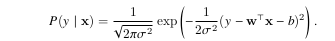
Let’s assume that observations arise from noisy measurements where the noise is normally distributed as follows

E is a noise term

Then the likelihood of getting a particular y of a given x is

According to the principle of maximum likelihood, the best values of parameters w and b are those that maximize the likelihood of the entire
dataset

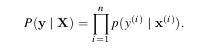
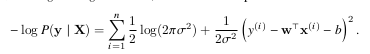
The final formula for minimizing the negative likelihood is as follows

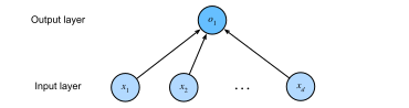
Finally, Linear regression is considered a single-layer neural network

And that’s all for section 3.1, it’s kinda intense but once you break it into smaller pieces, it’s enjoyable and easy.

Thank you for making it to the end of this article and will meet you in part 3!

BECOME a WRITER at MLearning.ai

Mlearning.ai Submission Suggestions